
Shape Models
An approach to image segmentation often used in computer vision is to provide the computer with knowledge of the objects that are expected to be visible in the scene. This approach is especially appealing in normal anatomy, since the objects are known. One of the reasons that radiologists must learn anatomy is that their prior anatomic knowledge helps them find objects in images. Therefore, we believe that if we can give the computer spatial knowledge of anatomy, it will be able to use this knowledge to help find structures in images.
For our purpose a spatial knowledge base will consist of a complete 3-D model of all normal anatomical structures, incorporating both the normal range of variation and the spatial relationships of these structures. Given such a model and associated knowledge-based imaging functions, it should be possible to create an instance of the model which conforms to a particular patient's anatomy, thereby segmenting the associated image set in the process.
For both our image segmentation and earlier protein structure work we have developed a representation, called geometric constraint networks (GCNs) [Brinkley1985,Brinkley1992], that attempts to model 3-D shape and range of variation by a set of interacting local shape constraints. The hypothesis behind this representation is that a collection of local constraints can interact to generate an ``emergent'' representation for the overall shape of the object.
Our more recent work (while at the University of Washington) was supported by the National Cancer Institute on a FIRST award to Jim Brinkley (1992-1997), and by the Achievements Rewards for College Scientists (ARCS). The work since 1992 has been done by Kevin Hinshaw, a Ph.D student in Computer Science.
For image segmentation we implemented and tested a 2-D version of GCNs called a radial contour model (RCM) [Brinkley1993a,Hinshaw1995] shown superimposed on a cross-section of the kidney in figures 1 and 2. The model consists of a set of fixed radials emanating from a local contour coordinate system, where a 2-D contour of an organ on an image is defined by the position along each radial to the organ border. Shape knowledge is represented by a set of local constraints between neighboring radials, where each constraint essentially specifies the range of allowable slopes for the line between neighboring radials.
The RCM was implemented within a semi-automatic knowledge-based image segmentation system called Scanner [Brinkley1993a,Hinshaw1995].
Figure 1. Screen snapshot of Scanner.
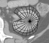
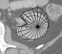
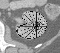
Figure 2. Fitting a radial contour model to the kidney.
Figures 1 and 2 are screen captures from Scanner, in which a set of 8 similarly shaped contours from the hilar region of the kidney were used as a training set for a RCM describing the shape and range of variation for a cross section of the normal kidney. To segment a new contour, the user indicates two endpoints of a long axis on the kidney cross-section. These points establish the location of the kidney model in the image, while also defining the lengths of two radials in the model. These distances are propagated throughout the network of constraints to generate the first model in figure 2, which shows an outer and inner boundary defining an uncertainty region, as well as a current ``bestguess'' boundary defined by the midpoint of each radial uncertainty interval. This model was generated solely from the two axis endpoints and the constraints learned from the training set.
The uncertainty region defines the range of instances that remain compatible with both the model and with the data that have been examined so far. In Scanner the uncertainty region is used to limit the search for the distance along each of the remaining radials to the edge of the kidney contour. For each radial an edge finder looks for the edge only along the interval defined by the inner and outer uncertainty contours. Once an edge is found it is propagated throughout the network, resulting in a smaller uncertainty region, which is then used to constrain the search for more radials. The middle image of figure 2 shows the model after several edges have been located and the bounds have been tightened. The procedure terminates when (1) all the radials have been examined or (2) the uncertainty area is small enough. The bestguess contour is then taken as the result. The last image in figure 2 shows the final stage in this process. Once the procedure terminates the user can correct any radials whose edges were incorrectly found.
The resulting 2-D contours can then be used as input to the 3-D reconstruction procedure.
The 2-D radial contour model was evaluated on 15 cross-sectional shapes from CT images of 16 patients, with the goal of decreasing segmentation time for radiation treatment planning, since the current method is mostly manual [Brinkley1993a,Hinshaw1995]. The evaluation showed that the RCM has the potential to decrease segmentation time by about a factor of 3 over a purely manual technique, for many of the ``critical'' structures that must be avoided during radiation treatment for cancer.
The advantage of this procedure over a pure edge following or region based approach is that the model can ``hallucinate'' edges where none are present in the image, a frequent occurrence with soft tissues or with noisy imaging modalities such as ultrasound. Our approach also recognizes that no current segmentation technique is error-free, so it necessary to include the user as an integral part of the process.
The advantages of the 2-D model, and its successful evaluation on 2-D data, have led to an implementation of a 3-D radial model [Hinshaw1996, Hinshaw1997].
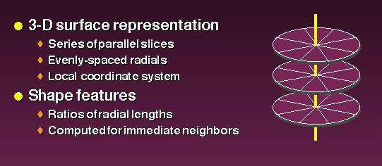
Figure 3. In this case the radial model is defined by a set of parallel slices through the organ, each of which is a radial contour model. Local constraints are applied not only within a slice as in the 2-D model, but also between slices, thereby allowing information obtained on one slice to reduce the uncertainty on adjacent slices.
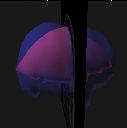
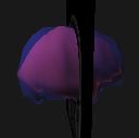
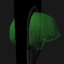
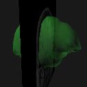
Figure 4. This figure shows four stages in the segmentation process, beginning with a radial model defined by finding an edge on one radial and propagating it to the other slices, and ending with the final model.
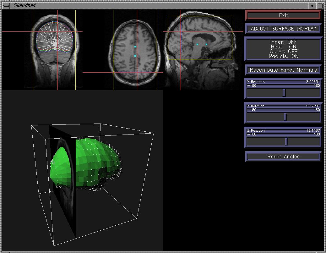
Figure 5. The 3-D model is implemented within a 3-D extension of Scanner.
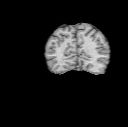
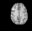
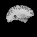
Figure 6. Since the radial model is not detailed enough to capture all the gyri and sulci in the brain it is used to generate a mask, in a similar manner to the 3-D region grower.
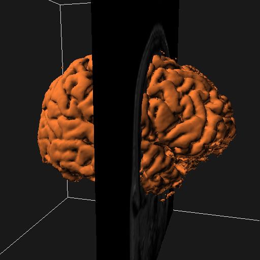
Figure 7. The mask is input to a similar surface-extraction scheme as in the region-grower.
We are in the process of using this technique to generate the 3-D renderings for the brain mapper.
However, the radial model cannot represent the detailed anatomy of structures such as the sulcal patterns on the brain surface in figure 7. The current search engine also has no way to restore an instance of the model that is eliminated by incorrect choice of an edge along a radial. On the other hand, the currently popular deformable models require a good starting structure in order not to become lost in a local minimum. Thus, one approach we are exploring is to use the radial model as a starting point for other techniques such as deformable models, edge or surface following, or region growing. The constraints can also be incorporated directly into the cost function of a deformable model, in order to provide additional shape knowledge to the adjustment procedure.
Once such shape models are developed for individual organs (e.g. kidney, liver), the models can be related to each other, so the position of one structure constrains the search for the other. However, representation of variation in the transform relating one 3-D coordinate system to another can be computationally intractable [Brinkley1988]. For this reason we have explored the possibility of probabilistic measures of variation [Altman1993a]. For the 2-D models there was no significant improvement over the minmax approach [Hinshaw1995]. However, in the 3-D case it is likely that the computational savings will make this approach the preferred method.
Last modified: Wed May 14 11:46:32 PDT 2003 by Kevin Hinshaw (khinshaw (at) u.washington.edu) by kph