Chapter 1

1.1 Motivation

Through the use of modern scanning and rendering technologies, it has become theoretically possible to reconstruct and render the anatomy of the human body at arbitrary levels of detail. However, at present the vast majority of applications utilizing this technology exist solely as research prototypes working on toy models or as vast modeling applications such as Maya[2] or 3D Studio MAX[1], designed with animators and game designers, rather than the anatomist, in mind. The goal of this thesis is to leverage and improve existing rendering and model construction technologies to create a powerful and easy-to-use suite of software tools designed to meet the needs of anatomists and students who wish to recreate digital models of the human body. Our software is capable of creating 3D models based on image data from the human body and designing complex scenes using these models. These scenes may later be used by students or anatomists to explore the structure of the human body.

Figure 1.1: Workflow diagram

Our pipeline for creating 3D scenes begins with the BodyGen program. At a high level, this tool allows users to create and save 3D model files in .obj format, a common 3D model description format, by specifying the model’s contours through a set of image data. With BodyView, a user can combine multiple models created with BodyGen to design complex scenes of the human body, e.g. combining many models from the brain together to form a scene depicting the human head. These scenes are then saved in VRML format. (See figure 1.1.)

1.2 Distinguishing Features of BodyGen/BodyView

Numerous pieces of commercial software currently exist to create 3D models and scenes based upon those models. The BodyGen and BodyView programs, however, contain rendering and geometric algorithms to solve problems that specifically arise in the creation of 3D models and scenes for biological purposes.

Problem 1: Unlike game or movie models, biological models are generally based upon sets of 2D images.

For this reason, traditional modeling packages based upon combining and modifying primitive objects such as cubes or spheres are not feasible. A new modeling approach, with contours as the primitive, is needed.

Solution: The BodyGen system has been specifically designed to deal with contour data as the basic modeling primitive used to create complex meshes.

A correspondence algorithm used to create groups of contours and a tiling algorithm used to create meshes based on these contours have been incorporated into the program. These features are not found in traditional modeling software packages.

Problem 2: Due to the need for high accuracy in the creation of models depicting human anatomy, objects with extremely large numbers of polygons result.

In a movie or game, the exact curve of a character’s nose may not be important. However, in anatomical models, every crease and bump must be meticulously modeled. This results in models containing vast numbers of polygons. To give an example, a set of models detailing the brain’s structure contains over 800,000 triangles. To interactively view scenes containing many objects of this nature, a method of managing complexity is vital. Traditional modeling applications do not allow the user to interactively control model detail.

Solution: We have incorporated a dynamic level of detail algorithm into the BodyView program.

This feature allows the user to create and interact with scenes involving highly complex models by reducing the level of detail in areas that are not of interest, while maintaining accuracy in areas that require greater detail.

Problem 3: In scenes involving anatomy, it is often desirable to view a specific object in the context of the entire human body.

Unlike movie or game models, biological scenes, especially those in textbooks, use hand-drawn figures mixing several different drawing styles to draw attention to areas of importance. Traditional modeling and scene generating packages do not allow the user to mix several rendering styles together to achieve this effect.

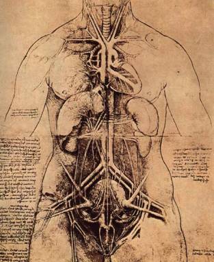
Figure 1.2: A sketch of the human stomach by Da Vinci

Solution: We have incorporated two hand-drawn rendering algorithms along with the traditional smooth-shaded rendering MeshView’s display technology.

Renaissance artist Leonardo Da Vinci often drew detailed sketches of human organs encased within a very roughly drawn human form to give the anatomical models a context. (see Figure 1.2) This approach gives the user freedom to create a context for the organs of interest in a low-detail, hand drawn style, while still rendering the desired objects in a realistic and highly-detailed fashion.

1.3 Chapter Overview

Chapter 2 presents the first half of our software suite, the BodyGen program, and describes in detail the algorithms involved. Specifically the correspondence and tiling algorithms required to deal with the image contours touched upon in Problem 1 above are described and demonstrated in the context of creating biological models. Chapter 3 describes the second half of our set of tools, BodyView. In this chapter the algorithms involving mesh decimation, or dynamic multiresolution, and hand-drawn rendering algorithms touched upon in problems 2 and 3 will be discussed. Finally, Chapter 4 summarizes our work and explores areas for further research.

Chapter 2

BodyGen

2.1 Overview

Planar contour data describing the outlines of organs in the human body have become easily obtainable in recent years. Examples of data that can be used to create these contours include the Visible Human Project[21], ultrasound, and magnetic resonance imaging (MRI). Through image segmentation techniques and hand tracing, accurate polygonal contours defining organs of the human body may be obtained from these data. Utilizing this contour information in the semi-automatic construction of complex surfaces is a vital step in creating highly accurate 3D models of the human body.

The goal of BodyGen lies in comparing existing techniques for the creation of these surface models from contour data, choosing the most promising methods, and integrating them together into an easy-to-use package that will be freely distributed. By utilizing this software, biologists from around the world will be able to generate three-dimensional models describing organs; these may be combined to create a freely available, highly accurate model of the human body.

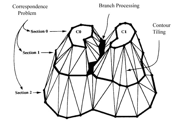
Figure 2.1: Illustration of the model creation process

2.2 Architecture

The construction of three-dimensional models from contour data can be broken into the following four steps

1. Contour Specification

2. Contour Correspondence

3. Contour Tiling

4. Branch Processing

BodyGen has been modularized to handle these sub-problems separately so that new techniques can be easily interchanged with the existing methods. The user may also solve these problems by hand, bypassing the automatic techniques entirely. A visual representation of these problems can be seen in Figure 2.1.

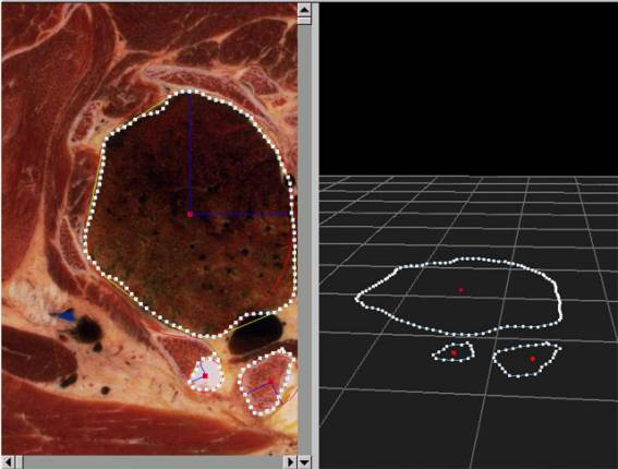
Figure 2.2: A screenshot from BodyGen illustrating contour drawing

2.3 Contour Specification

The contour data utilized by BodyGen is based upon a set of images. Each image is considered as a planar surface separated from the previous and next layer by a constant distance. The first step therefore lies in determining the position and boundaries of organs of interest in the image. Due to the complexity of biological images, manual contour specification is currently the method of choice for defining contour placement in these images. Figure 2.2 illustrates the creation of contours specifying portions of the lung and two secondary organs in a single image.

2.4 Contour Correspondence

Once a set of contours in each image has been determined, it becomes necessary to determine which of these contours specify individual models. The goal of the Contour Correspondence step of BodyGen lies in automatically determining a set of contours, which when combined, form an anatomical model.

2.4.1 Previous Work

The first work in this area by Soroka [20] used contour overlap between level i and level i+1 to determine the correspondence in contours between neighboring levels. Bresler et al. [4] fitted generalized ellipses to each contour, then used these ellipses to create generalized cylinders based upon the contours. They define the “best correspondence” by the generalized cylinder that possesses the smallest deviation from a perfectly linear generalized cylinder, or a cylinder whose axis defines a perfectly straight line. This approach, however does not take into account similarity of shape between neighboring ellipses, and does not work well for contours whose shape is not well approximated by an ellipse.

The most recent advance in Correspondence and the method used in this project is a Graph-Based Technique. Skinner [6] and Shelley[19] attempted to solve the correspondence problem by redefining it as a shortest-path graph problem. In this method, for each contour in level i and level i+1, a best-fit ellipse is found. Next a 5-tuple is determined for each ellipse. This 5-tuple is defined as (x_c,y_c,q,a,b), where x_c and y_care defined as the coordinates of the best-fit ellipse’s center, a and b are 2d scaling vectors defining the best-fit ellipse’s major and minor axes, respectively. Finally, q represents the deviation of the major and minor axes from the vertical position. A graph is then created between every contour in level i and every contour in level i+1, where the weight of the edge between contour A and contour B is equal to the Euclidian distance between the 5-tuples describing the fitted ellipse of each contour. The correspondence between the contours in level i and level i+1 is then determined by finding the minimum spanning path through this graph. The links between the contours on the same level are discarded, after which, the links in this minimum spanning tree connecting level i, from level i+1 define contour correspondence.

2.4.2 Implementation

In our implementation of the Correspondence problem, we have utilized a modified version of Skinner’s minimum spanning tree algorithm. However, in our version of this algorithm the edge weight between two contours A and B is defined as the weighted sum of the Euclidian distance between the respective 5-tuples of A and B, as defined above, and the average of the percent of area overlapped between the projection of contour A onto contour B and conversely B onto A. In this way the methods of Skinner and Soroka are combined to give improved results.

Stated more succinctly, the weight between Contour A and Contour B is defined as follows:

W_AB = xD + yO

where:

x + y = 1

D = Euclidian distance between 5-tuple_Aand 5-tuple_B

O = 2/(Overlap(A,B) + Overlap(B,A) )

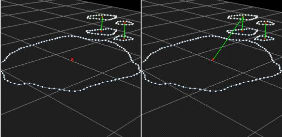
Figure 2.3: (L) Implemented algorithm (R) Original Skinner algorithm

The scaling factors, x and y, are determined for each contour pair individually as follows:

x = (Overlap(A,Ellipse(A) ) + Overlap(B,Ellipse(B)) / 2

y = 1 – x

In this way, when the ellipse represents a good fit to the contour, the similarity in ellipse shape and position in the 5-tuple is used as the matching parameter. Conversely, when the ellipse is unable to capture the contour shape, we rely mainly on overlap to determine correspondence. A second deviation from Skinner’s algorithm lies in the requirement we make of the minimum cost spanning tree. Skinner required that all nodes be visited at least once in the correspondence mapping. As can be seen in Figure 2.3, this will automatically create branches in cases where the number of contours in plane i differs from that of i+1. We have found that in complex scenes the algorithm fails to correctly identify branching points, requiring user interaction to correct the mistakes. For this reason, we require that the minimum path only pass through each contour of the plane containing fewer contours. This eliminates any need to predict contour branching and entrusts this task to the user.

2.5 Contour Tiling

The tiling step composes the core of BodyGen. Stated briefly, the goal of this stage is to create a triangulation, referred to as a ribbon, between a single contour present in image plane i and a single contour in image plane i+1 such that each vertex of the two contours is present in two of the triangles which compose the ribbon. Our criteria for determining a “good” tiling method relies on the following criteria:

1. The method must be able to create tilings for contours that differ drastically in shape.

2. In the field of biology, high precision will often be desired. This will result in high vertex counts, and, as a result, our tiling method must be fast even for complex contours.

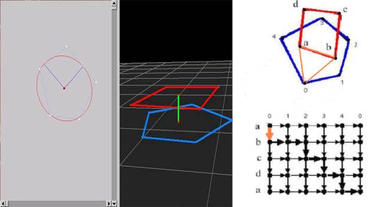
Figure 2.4: A tiling algorithm example, Pt. 1

2.5.1 Previous Work

The bulk of previous work in the area of contour tiling focuses on optimization based approaches. The first optimization-based approach was proposed by Keppel [13]. In this method, a two-dimensional graph is created from the vertices of each contour as can be seen in Figure 2.4. The vertices of the upper contour, composed of vertices <a,b,c,d>, define the rows of this graph, while the vertices of the lower contour, composed of vertices <0,1,2,3,4>, defines the columns. Figure 2.4 illustrates this situation.

In the graph of Figure 2.4, each edge defines a single triangle between the upper and lower contour. This triangle’s vertices are defined by the unique row and column numbers in the graph edge coordinates. As an example, the edge (0,a) to (0,b) would define a triangle defined by vertices 0, a, and b. Finally, the weight of each edge is determined by the area of the triangle that it specifies. weights, a tiling is found by determining the lowest cost path from the upper left to bottom

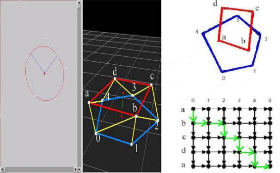
Figure 2.5: A tiling algorithm example, Pt. 2

right corner of the grid. This process is illustrated in Figure 2.5.

However, the main drawback of this approach lies in its slow speed, O(a²+b²) for a pair of contours with a and b vertices respectively. Fuchs et al. [8] improved upon this algorithm by employing a Divide-and-Conquer style algorithm to increase the optimization speed. Their approach reduced the running time of the algorithm to O( ab log (max(a,b)) ).

The research of Meyers et al. [14] first introduced multiresolution into the tiling problem. Their approach utilized a multi-resolution method to reduce the optimization time even further. Stated briefly, a wavelet filter is passed over each contour until the contour has been reduced to a predetermined number of vertices. Fuchs’ algorithm is then performed on this simplified contour to create a mesh based upon the simplified contours. Finally, detail is added back to the simplified contours, with local optimization performed when each vertex is added, until, the original contours are achieved. The overall running time for this algorithm is equivalent to:

O(m² log m) + O(max(a,b) log max((a,b)) )

where, m=# of vertices at the lowest resolution

The first term of this equation simply represents the running-time of Fuchs algorithm for the simplified contour. The running time to add a single vertex and perform local-optimizations is equal to log(n), which must be performed for each contour vertex that had been removed by the simplification process. This results in the O(a log n) term as seen above, where a represents the total number of vertices removed during the simplification process and n represents the total number of vertices in the model.

The most recent development in the area of contour tiling is from Barequet and Wolfers. [3] In this research a linear time algorithm is found for tiling two contours with similar shape characteristics. A method is also proposed for automatically modifying the contours’ shapes to force these shape similarities. This is currently the fastest tiling algorithm available. However, it is not useful in our application as it requires that the input contours be modified, an unallowable step as anatomical models’ contours must remain faithful to the original image data.

2.5.2 Implementation

The method chosen for implementation in BodyGen is a modified version of the Meyers et al. multi-resolution tiling approach. This is currently the fastest and

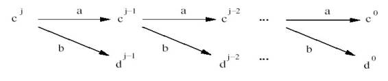
Figure 2.6: A graphical representation of the filter bank

most accurate tiling algorithm available today for use with unmodified contour data. The exact procedure is briefly sketched below, followed by a more detailed section describing each step and divergences from Meyers’ original method.

1. Utilizing wavelet filter banks, find a low-resolution version of the original contour.

2. Utilizing the Fuchs algorithm, perform a low-resolution tiling for the simplified contours.

3. Replace removed vertices one at a time, performing local-optimization over the affected area at each step.

The first step of this procedure requires the creation of a coarse model that approximates the original contour. We follow Meyers’ use of the wavelet filter bank method for this step. The filter bank method guarantees that the shape of the low-resolution contour will minimize the least-squares error between the course and original model. The method works as follows.

At each step the set of contour vertices c^j is multiplied by a filter kernel and a detail kernel. As shown in Figure 2.6, this results in two vectors, c^j-1and d^j-1. c^j represents the contour vertices at resolution level j, d^j-1 can be thought of as storing the information necessary to retrieve the more detailed contour data c^j from contour vertices c^j-1. A full analysis of the mathematical properties of wavelets is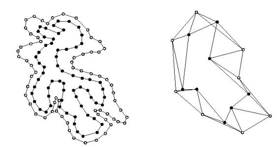

Figure 2.7: Left: Full Contour, Right: Tiled, Coarse Contour

beyond the scope of this paper. The reader may find more detailed information on this approach and definitions of the detail and filter kernels in Chui [5].

Following the creation of these simplified contours, the Fuchs algorithm is performed to find an optimal tiling, as shown in Figure 2.7. Our optimization criteria is triangle surface area, giving rise to tilings possessing minimum surface area. The output of this algorithm is a set of triangles connecting the two simplified input contours.

The final step in our tiling implementation lies in adding detail back to the course representations to achieve a tiling of the original contours. This is achieved by multiplying the detail vector d^j-1 by the inverse detail kernel, and adding the result to the simplified contour, c^j-1.

Figure 2.8: Circles represent newly added vertices.

In short, this step adds one additional vertex per triangle edge, converting the each triangle to a quad. (see Figure 2.8) For each added vertex, we now have a choice of changing the triangulation of the newly created quadrilateral by swapping an edge. This decision is based upon the same triangle surface area cost function as used in Fuchs algorithm. When a new level of detail is added each legal edge swap is performed and it’s change to the overall cost is determined. If the swap results in a decrease to the cost function, the swap is performed, changing the tiling, and all newly legal edge swaps are tested to see how they modify the cost function. This procedure is continued until there are no longer any swaps which will lower the cost function. At this point the next level of detail is added to the contour and the procedure is repeated. This continues until we have returned to the original contours. A screenshot from BodyGen in Figure 2.9, illustrates a set of initial contours and the resultant tiling.

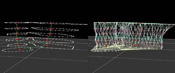
Figure 2.9: A completed tiling

2.6 Contour Branching

There are many instances in which body structures will branch and perhaps later re-merge, giving rise to the branching problem. Stated more precisely when the number of contours in image I_a is not equal to the number of contours in image I_a+1, a branch has occurred or one or more contours have ended. Our goal is to create visually appealing tilings in these cases.

2.6.1 Previous Work

The previous research in this area can be broken into two main areas, that of composite contour algorithms, and medial axis algorithms. The first use of composite contour algorithms was by Christiansen and Sederberg [6]. We will use the terms PreBC and PostBC as follows: PreBC defines the single contour which exists in an image plane previous to the branch. PostBC defines the set of contours that exist after the branch has occurred. The approach of Christiansen et al was to combine all contours in the PostBC set into a single contour by locating the contour pairs between PostBC of minimal distance and connecting them, thereby creating a single contour whose shape is loosely defined by the PostBC. Tiling is then performed on these two single contours as described in the previous section with triangles whose vertices span two or more contours discarded. However, there exists one large problem to this approach, the Composite Contour does not always accurately capture the shape of the set of PostBC contours, resulting in unappealing tilings. (see Figure 2.10)

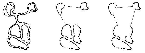
Figure 2.10: Naïve Branching Algorithm Example

Left-The original contour, Center-Closest Points between contours found, Right- The 5 PostBC elements are combined into a single contour.

Meyers [9] proposed a novel scheme for handling branching contours utilizing the medial axis of the PostBC projected onto the PreBC. The medial axis is a special case of Voronoi diagrams for surfaces containing holes. Stated succinctly, the medial axis (MA) is defined as the set of points whose distance from any two points on the Pre or PostBC is equidistant. The MA is used to both define a mapping between the PreBC and the PostBC, and create multiple new PreBC, one for each element in the PostBC set. These pairs of contours are then sent to the tiling engine for mesh creation. Each point in the MA is defined by two points on either the PreBC or an element of the PostBC set. Sections where both points lie on a PostBC, are used to split the PreBC into a number of contours equal to the number of contours in the PostBC set. A simple example will clarify this greatly. In this case there are two contours in the PostBC set.

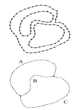
Figure 2.11: Top-Original Contours Bottom-Medial Axis Derivation

The MA for the contours shown above in Figure 2.11 can be broken into three components, A, B, C. Sections A and C, represents a portion of the MA that defines a correspondence between the Pre and PostBC. In contrast, section B, is defined by points from the PostBC elements. Section B is used to split the PreBC into two contours by finding the vertices closest to the MA branch points, and connecting them to this section, thereby creating two contours. Sections A and C define which of the new contours from the PreBC correspond to the PostBC elements. These pairs of contours are then input to the tiling engine for meshing, thereby creating a true branched surface.
The drawbacks to this method however lie in the extremely slow speed of

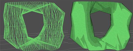
Figure 2.12: Branching Implementation Example

the medial axis derivation. This algorithm runs in O(n⁴) time and takes approximately 16 minutes to create the medial axis for a contour composed of 904 vertices on a PIII 500Mhz processor, making this approach unfeasible for interactive applications.

2.6.2 Implementation

While producing visually pleasing results, the lack of interactivity prompted us to abandon Meyers scheme for producing branching surfaces and utilize a much simpler approach. Our current approach to the branching problem makes use of the observation that in many cases the separation between image planes is very small, meaning that the impact of any one ribbon is nearly insignificant in the visual appearance of the entire structure. For this reason, we solve the branching problem by independently finding tilings between each pair of contours in the pre and post branch contour set and displaying these overlapping tilings to the user. This approach results in an unnatural cross-section when the models are cut.

However, the technique is fast and the external appearance is quite acceptable. (see Figure 2.12)

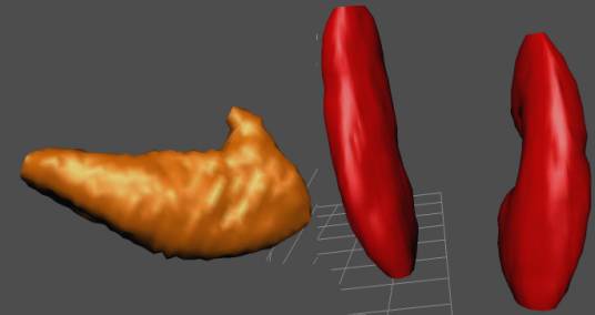
Figure 2.13: Right-Gall Bladder, Left-Left and Right Kidneys

2.7 Results

In this section we will discuss the actual usage of the BodyGen software and show examples of actual anatomical models created using the system. For the purpose of testing our software on real users and beginning the process of creating detailed anatomical models of the human body, two part-time users have been employed. These test-users have created ten detailed anatomical models based upon the Visible Human data set using the BodyGen software exclusively. These models include the human spleen, lungs (r and l), kidneys (r and l), gall bladder, radias ulna (r and l), and left clavicle (r and l). The average creation time for a model was largely dependent on the size and complexity of the model contours; the average time was three hours per model. The most complex of these models were the right and left human lungs due to their large size. Composed of over 200 images, the lung models required approximately six hours to create. Figures 2.13, 2.14, and 2.15 depict a sampling of the final anatomical structures created with the BodyGen program.

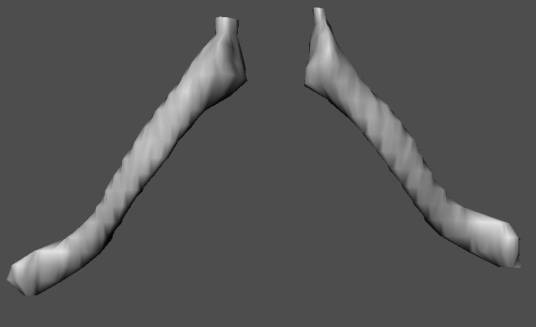
Figure 2.14: Left and Right Clavicle

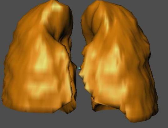
Figure 2.15 Right and Left Lungs

Chapter 3

BodyView

The goal of the BodyView program is to allow biologists to quickly and efficiently create complex scenes of the human body involving numerous models of the human body. We will first discuss the overall architecture of the BodyView system, then look more closely at the dynamic multiresolution and non photo-realistic (NPR) rendering algorithms.

3.1 Overview

Scene generation programs are not at all uncommon in the computer graphics field. SGI’s OpenGL Inventor[18] was the first scene description program, allowing users to position, texture, and shade imported polygonal objects. The scene description file format for Inventor became the basis for the VRML[22] description language, currently the most widely used scene description langauge. Numerous 3D modeling packages, such as Maya and 3D Studio Max, have also advanced the area of scene description by including higher level primitives such as subdivision and NURB surfaces to the primitive object types, as well as including rigid-body dynamics to simulate the motion of the objects present within the scene. All of these previous efforts, however, have large drawbacks when being used with biological models.

Beginning with the Inventor and VRML based scene-creator tools, an immediate problem that arises is the lack of functionality needed to manage the complexity of present biological models. These programs allow users to modify the exterior properties of a model, such as texture placement, and interior properties such as vertex positions. However, they provide no capabilities for dynamically and automatically creating simplified versions of a model. For example, individual vertices of a brain model composed of two hundred thousand polygons could be modified. However, an accurate version of the model containing only five thousand vertices would require tremendous manual effort, requiring the user to delete and reposition countless vertices. In modern rendering packages, such as Maya, the reverse problem occurs. The functionality needed to create scenes as well as reduce and restore detail in models is present, however the user is overwhelmed by the functionality present in the program, and must spend many weeks learning the tool. In addition, these modern tools are designed purely for the scene creator, e.g. artists who wish to create scenes that will be viewed in a movie or game. For the novice user who desires only to view and manipulate scenes at the basic level, they are prohibitively expensive and complex. Finally, all current scene description programs lack rendering options that include hand-drawn styles.

The BodyView program was created specifically to fill a gap present in current scene description programs. Our goal was to create a program usable both by anatomists, to create complex scenes involving detail anatomical models, and by students who would wish not to create scenes, but to view and interact with those already created. To manage the complexity involved in anatomical models, we have incorporated an easy-to-use level of detail interface for the user, allowing

Figure 3.1: Importing a Model

a scene creator to display an object with only as much geometrical information as is needed, as well as two hand-drawn rendering algorithms, which allows a user to create contrast and emphasis to a scene as he or she sees fit.

3.2 Architecture

As with any 3D scene authoring tool the basic data structure in our program involves a collection of 3D objects, which the user loads in individually as .obj files, or as pre-created scenes in the form of .vrml files. Once loaded, the user may modify the position, orientation and grouping of the objects, as well as initially set the model’s level of detail and rendering style. (See figure 3.1.)

Once a model is loaded, the rendering options are set via a drop down box. These options include Wireframe, Smooth Shading, Hand-Drawn 1, and Hand-Drawn 2. The specifics of our hand-drawn styles will be discussed in a later section. The model’s level of detail is set through a discretized slider bar. The bar is divided into ten regions, n1-n10, each representing a model containing 10% fewer polygons than the last. For example, n10 represents a model containing 100% of the original model’s polygons, whereas n4 represents a model containing 40% of the polygons from the original. These properties may be modified at any time for any model.

In addition, we have implemented a group-level properties command allowing the user to modify the rendering style or level-of-detail for an entire group. Each model imported into BodyView is a member of a user-determined group. By selecting the Group Properties option, the user may raise or lower the level of detail, or set a rendering option for all members present in the group at one time. This functionality is useful for both the scene creator and the student, as it allows the user to quickly highlight an area of interest.

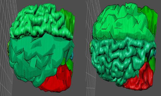
Figure 3.2: Modifying Group Properties

For example, if a student had finished studying the right brain and was prepared to move into a study of the left brain’s anatomy, he or she could quickly scale down the detail for all members of the right half and set its rendering style to hand-drawn. This would provide a low resolution and non-distracting reference for the brain study. The student could then raise the resolution of the left brain models to full-detail and change its render setting to smooth, which would allow for a detailed view of the brain’s workings. (See figure 3.2)

3.3 Multiresolution

In this section we will explore previous work in the area of level-of detail as well as examine the multiresolution algorithm used in the BodyView program.

3.3.1 Previous Work

Level of detail control or mesh decimation is not a new area in computer graphics. The simplest and most straight-forward approach, that of discrete multiresolution [9], has been in use since 1993. In this approach an artist creates multiple versions of a single model at varying levels of detail using a 3D modeling tool such as Maya or 3D Studio Max. At run time, the program will then decide which of these pre-built models to use based on user-input or current frame-rate. This technique does not require any algorithmic manipulation of the model’s geometry, as the artist has already supplied the necessary low-resolution models. The rendering engine must simply choose which version of the model to display at a given frame. Although this is the simplest solution to the multi-resolution problem, serious drawbacks are present in the realm of anatomical modeling. Using this technique, an artist must manually create low-resolution models for every object used, a daunting task when dealing with the thousands of structures in the human body. Additionally, each model version must be stored in memory, a prohibitively expensive task when dealing with models which may reach millions of polygons, equating to tens of megabytes in size.

A second approach is that of wavelet analysis [7,11]. In this approach, each surface is constructed using a wavelet basis, e.g. each vertex position is specified by the summation of a series of Fourier cosine functions. The mesh is then decimated to the desired level of detail using signal processing methods. This method can produce highly accurate low-resolution models. However, as stated previously the surface must be reconstructed, or remeshed to meet certain restrictions before the wavelet analysis may continue. This approach modifies and introduces error into the highest level of detail in our model, making it less than ideal for biological models that have been painstakingly created with every polygon in the correct location. In addition, the wavelet representation is also unable to faithfully preserve sharp corners at lower levels of detail.

The final method of multiresolution, and the one used in our work, involves the use of cost functions and edge contraction. [10, 12, 15] In this technique, a cost function evaluates the effect of removing each vertex from the mesh. Two vertices containing the lowest cost functions, in other words, two adjacent vertices whose removal would modify the mesh’s structure the smallest amount, are chosen from a pool of candidates. The edge formed by these two vertices is then collapsed by taking the two chosen vertices and moving both to an average position, typically removing two triangle faces per operation. This group of algorithms work by iteratively selecting edges for deletion, collapsing the edge and modifying the resulting model’s edge connections accordingly. The main difference in these algorithms lies in the selection of a cost function or how the particular edge to be contracted is chosen. Although these methods are generally less accurate than wavelet algorithms, they are faster and can work directly with the original model’s mesh.

3.3.2 Implementation

This brings us to the level-of-detail method present in the BodyView software. We have chosen to implement the level-of-detail (LOD) described by Garland and Heckbert [18]. This algorithm is of the cost function variety and for reasons stated above is the best fit for our anatomical models. In this section we will

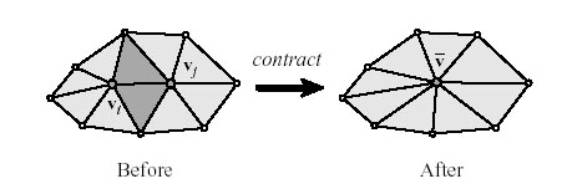
Figure 3.3: Example of edge contraction.

outline the exact procedure by which our low resolution models are created using this technique.

As described previously, this method works by continually selecting optimal vertices for removal at each step. It is a “greedy” algorithm as it is concerned only with the optimal vertices at the current step of the algorithm and not how the collapse of the associated edge affects previous or future choices. The flow of the algorithm is as follows (See Figure 3.3):

1. Compute the value of the cost function for each connected vertex pair in the model (this step is costly and performed only once)

2. Select a pair of candidate vertices.

3. Contract this pair of vertices (v_i,v_j) by the following method:

a. Average the positions of v_i and v_jand create a new vertex in that position.

b. Update the edge connectivity of all triangles previously connected to v_iand v_j.

c. Remove all degenerate triangles. (those with less than 3 unique vertices)

d. Update all cost functions that have been modified as a result of this step. (Usually this is only a small number)

4. Repeat 1-3 until the desired level of detail is reached.

The final piece of this algorithm is the choice of the cost function for each vertex. We have followed Heckbert and Garland by selecting a cost function which measures the sum of the perturbation of the normals that would result if a vertex were moved. In the example show in Figure 3.3, vertices v_iand v_j each participate in six triangles in the Before configuration and 7 triangles in the After configuration . Our cost function is the sum of the differences between the normal values of these triangles in the Before and After configurations. For the purpose of speed we represent the set of cost functions as a min-heap. This data structure allows us to find the vertices with minimum cost functions in linear time and retrieve them from the heap in constant time.

3.3.3 Results

Using this approach, we are able to dynamically compute the removal of up to one hundred thousand triangles in less that one second. Figures 3.4, 3.5, and 3.6 illustrate this approach in action.

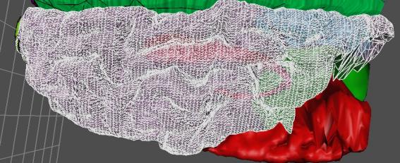
Figure 3.4: Brain model containing 98,123 triangles

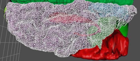
Figure 3.5: Brain Model containing 45,453 triangles

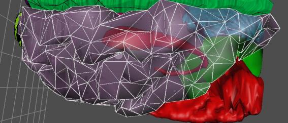
Figure 3.6: Brain Model containing 8,231 triangles

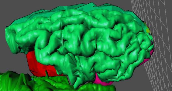
Figure 3.7: High Resolution Smooth Shaded Brain

3.4 Non-Photorealitic Rendering

A second major component of our system lies in the ability to perform non-photorealistic rendering of biological objects. The advantages of this approach are two-fold. The need for low-resolution models when dealing with scenes of anatomical objects is a given. Generally these low resolution models look quite visually unappealing and not realistic as anatomical objects due to our expectations of what realistically shaded objects should look like. The NPR style, however, provides a quite visually pleasing alternative at lower resolutions to the traditional flat-shaded approach. (See Figure 3.7, 3.8, 3.9)

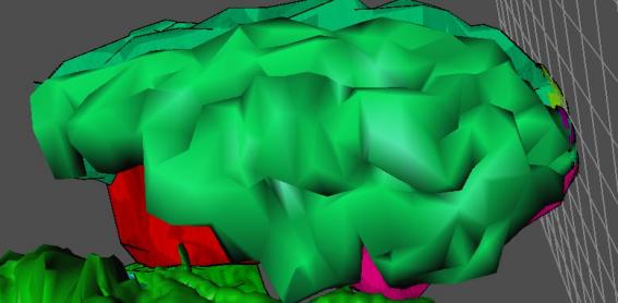
Figure 3.8: Low Resolution Smooth Shaded Brain

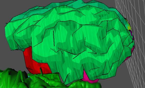
Figure 3.9: Low Resolution NPR Shaded Brain

The two main technologies used in conjunction to achieve this effect are silhouetting and texture blending algorithms.

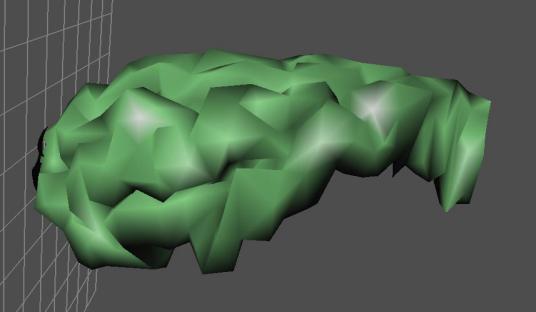
Figure 3.10: Smooth Shaded Brain

3.4.1 Silhouetting

Silhouetting is a technique used by artists for centuries to create a sense of shape and texture, while using as few strokes as possible. Ideally, the silhouette of an object should convey all of the necessary shape and geometry information of an object without the need for additional shading or texturing. In our program, an object’s silhouette is made up of two distinct parts, depicted in Figure 3.11 and 3.12 on the following page. Figure 3.10, showing the basic flat-shaded object, is given for reference. The first section of the silhouette is composed of a set of lines describing the boundary of the object when projected into the 2D viewing plane. The second set of lines is composed of the set of triangle edges shared between two or more triangles whose surface normal values differ greatly. The first component of the silhouette, or boundary lines, describes the rough shape of the object, while the finer geometry information is conveyed by the second component, detail lines.

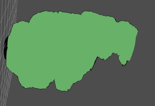
Figure 3.11: Brain boundary lines

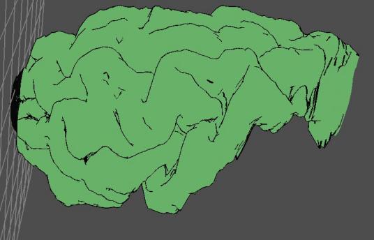
Figure 3.12: Brain silhouette - boundary lines + detail lines

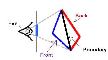
Figure 3.13: Graphical depiction of boundary line detection.

In the detection of these boundary lines, we use Zhang’s Backface Culling algorithm [23]. Expressed mathematically, the boundary lines of the silhouette are found by locating all triangle edges in which one triangle sharing that edge is front facing (facing the camera), and one triangle is back-facing. This can be expressed mathematically as:

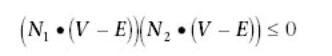
where N₁ and N₂ are the 3D normal vectors of the front and back facing polygons respectively, V represents one of the vertices from the selected edge and E represents the camera, or eye, position. When we have detected an edge that satisfies this property, we redraw it using a dark line to distinctly display the silhouette. This concept is illustrated graphically in Figure 3.13 above.

To generate the detail lines of the silhouette, we use an algorithm conceived by Raskar and Cohen [17]. This algorithm operates by finding the set of edges shared by two triangles whose surface normal angle varies by more than a predetermined constant, in this case, 45 degrees. A large variation in normal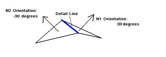

Figure 3.14: Detail Line Detection

orientation between two triangles indicates a rough or uneven section of the model.

As the purpose of the detail lines is to represent this type of geometric information,
we draw edges with this property in the same bold style as the boundary lines. (see Figure 3.14)

3.4.2 Multi-texture Hatching

Now that we have rendered the geometry in a hand-drawn style, the next goal in the creation of a hand-drawn rendering style is to artistically recreate the interplay of light and shadow on our objects. The technology used to achieve this hand-drawn effect is multi-texturing, a technique in which two individual textures are blended via an alpha map to create a final texture which is then pasted to an object. We leverage this technology to create an alternative drawing style to realistically smooth shading. When drawing rough sketches of objects, artists often use the convention known as hatching to simplistically illustrate light and shadow. The two main techniques in this approach are binary and discrete hatching. In the binary case, hatching is used when an object is in shadow and not used when in light. The discrete case is slightly more complicated and uses

Figure 3.15: Left-Discrete Hatching, Right-Binary Hatching

hatching density to create the illusion of shadow. Areas not touched by light are denoted by a dense hatching pattern, while those in light are depicted using a light hatching pattern. (see Figure 3.15).

This technique of multi-texturing to achieve this aritistic effect was first used by Lake et al, followed shortly by Hoppe et al. [16, 25]. In an interactive program such as BodyView, speed and responsiveness in manipulation of the models is an important goal. Due to its fast rendering speed on modern hardware, we have chosen to implement the multi-textured hatching algorithm put forth by Lake et. al. to achieve our non-photorealistic effect. We explain the details of this algorithm and show examples produced by our program below.

The Lake hatching algorithm mimics the continuous technique described above to depict light and dark areas on the model. First, a texture map representing each level of hatching is loaded. The BodyView application uses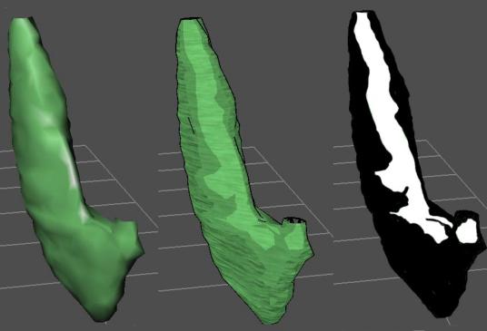

Figure 3.16: Multitexture Hatching Example

Left-Original Smooth Shading, Center-Hand-Drawn Rendering,

Right-Alpha Map for Texture Two (Alpha=1-White, 0-Black)

two texture maps for the sake of speed as this is currently the optimal number for most current graphics hardware pipelines.

Next, an alpha map is created based upon the lighting of the model at each frame in the following manner. (see Figure 3.16) The dot product between the light vector and the normal for each triangle in a model varies continuously between 0 and 1. Values less than 0 represent back-facing polygons and are not included. This value is used to determine the alpha value of each texture for that vertex using a thresholding approach. Vertices with a light dot product less than .5 are assigned an alpha value of 0 for texture one and an alpha value of 1 for texture two. Vertices with dot products between .5 and 1 are conversely assigned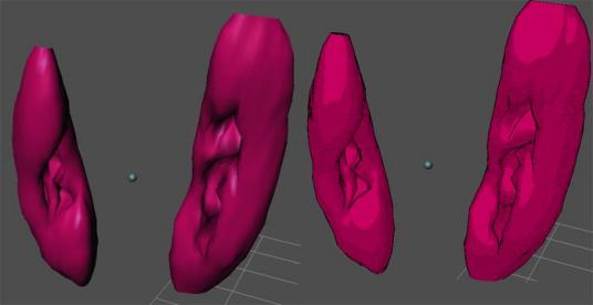

Figure 3.17: Left-Smooth Shaded Kidneys, Right-NPR Kidneys

an alpha value of 1 for texture one and 0 for texture two.

The light dot product value is used as an indicator to essentially turn on and off individual textures for each vertex. From an artistic standpoint this is the correct approach, as we would like to use different hatching to represent light (high light dot-products) and dark (low dot-products) areas. For neighboring vertices with differing alpha values, we linearly interpolate the alpha value across the triangle edge in the same fashion as Phong shading. To illustrate this technique on real data, the human kidneys, created with the BodyGen application, are depicted below in both a smooth and hand-drawn style. (see Figure 3.17)

Chapter 4

Future Work and Conclusions

4.1 Conclusions

We have developed a robust package for semi-automatically creating three-dimensional models from images slices and subsequently creating complex scenes using these models. The BodyGen and BodyView programs implement and combine the following existing key technologies to achieve this goal:

-Tiling of piecewise linear contours (BodyGen)

We have implemented a modified version of Meyers’ multi-resolution tiling algorithm to create triangulations between two piecewise linear contours. This technology allows us to quickly create three-dimensional anatomical models based upon a set of user-specified contours.

-Contour Correspondence Algorithm (BodyGen)

We have developed a new version of the correspondence algorithm, taking into account the accuracy with which best-fit ellipses match the original contours’ geometry when correspondence predictions are made. This algorithm is used to automatically predict which sets of contours should be triangulated using the above tiling algorithm to create an anatomical model.

-Multiresolution Meshes (BodyView)

We have implemented a version of Garland’s cost-function-based multiresolution mesh-generation algorithm to automatically create simplified yet accurate versions of complex anatomical models. At run-time, the user is able to create these simplified meshes in real-time based upon the requirements of the current scene and the available processor speed.

-Non-Photorealistic Rendering (BodyView)

We have implemented a NPR rendering scheme based upon Lake’s hatching algorithm. This feature allows the user to modify the display characteristic of individual anatomical models at run-time. This technology can be used in conjunction with the above multiresolution meshes to create a contrast between low detail background models, added to a scene to create context, and high detail foreground models, those which are the topic of study or inspection in a given scene.

It is the hope of the author that this program will be of use to biologists in the future as we work towards accurately digitizing and viewing the human form.

4.2 Future Work: BodyGen

4.1.1 Medial axis generation

Meyers utilization of the medial axis would be much more attractive if interactivity could be obtained while using this method for branch handling. For this to become possible, additional computational geometry research involving the efficiency of algorithms for generating the medial axis of polygons containing holes will be necessary.

4.1.2 Image Segmentation of Contours

Currently, one of the most tedious areas of the BodyGen program is the generation of contours. The user must draw each contour by hand and manually modify the contour vertices to accurately reflect the image data. Adding automatic image segmentation to this process would greatly simplify the user’s task.

4.2 Future Work: BodyView

4.2.1 Soft Body Physics Simulation of Surfaces

After three-dimensional surfaces have been generated, the next step is interaction with these images. The BodyView program allows users to name, orient and change the viewing properties of anatomical models. However, in areas such as surgical simulation, a more holistic interaction is necessary. For these type of applications users will need to poke, prod, and cut anatomical models, making the use of soft-body physical simulation a necessity.

4.2.2 Adaptive Multiresolution Meshes

Currently the program user is responsible for specifying the detail level for each anatomical model. Creating an automatic metric to modify the detail level of individual models based upon criteria such as polygon count, render time, and processor speed to maintain a constant frame rate regardless of viewing angle or scene composition would increase the ease-of-use of the BodyView application.

BIBILIOGRAPHY

[1] 3D Studio Max. http://www.discreet.com/.

[2] Alias-Wavefront Maya. Maya. http://www.aliaswavefront.com/.

[3] G. Barequet and B. Wolfers. Optimizing a strip separating two polygons. In

Graphical Models and Image Processing. 60(3):214-221, May 1998.

[4] Y. Bresler, J.A. Fessler, and A. Macovski. A Bayseian approach to

reconstruction from incomplete projections of a multiple object 3d doman.

In IEEE Trans. Pat. Anal. Mach. Intell., 11(8):840-858, August 1989.

[5] C. K. Chui. An Introduction to Wavelets. Academic Press, Inc.,1992.

[6] H.N. Christiansen and T.W. Sederberg. Conversion of complex contour line

definitions into polygonal element mosaics. In Proc. SIGGRAPH, pages

187-192, 1978.

[7] M. Eck, T. DeRose, T. Duchamp, H. Hoppe, T. Lounsbery, W. Stuetzle.

Multiresolution Analysis of Arbitrary Meshes. In Proc. SIGGRAPH, pages

173-182, 1995.

[8] H. Fuchs, Z.M. Kedem, and S.P. Uselton. Optimal surface reconstruction

from planar contours. In Communications of the ACM, 20(10):693-702,

October 1977.

[9] T. A. Funkhouser and C. H. Sequin. Adaptive Display Algorithm for

interactive frame rates during visualization of complex virtual environments.

In Proc. SIGGRAPH, pages 527-534, 1993.

[10] M. Garland and P. S. Heckbert. Surface Simplification using quadric error

metrics. In Proc. SIGGRAPH, pages 209-216, 1997.

[11] S. Gortler and M. S. Cohen. Variational Modeling with Wavelets.

Technical Report CS-TR-156-94, Dept. of Computer Science, Princeton

University, 1994.

[12] H. Hoppe, T. DeRose, T. Duchamp, J. McDonald, and W. Stuetzle. Mesh

Optimization. In Proc. SIGGRAPH, pages 19-26, 1993.

[13] E. Keppel. Approximating complex surfaces by triangulation of contour

lines. IBM J. Res. Develop., 19:2-11, January 1975.

[14] D. Meyers, S. Skinner, and K. Sloan. Surfaces from contours. In ACM

Transactions On Graphics, 11(3):228-258, July 1992.

[15] J. Popovic and H. Hoppe. Progressive Simplical Complexes. In Proc.

SIGGRAPH, pages 217-224, 1997.

[16] E. Praun, H. Hoppe, M. Webb, and A. Finkelstein. Real-time Hatching .

In Proc. SIGGRAPH, pages 581-586, 2001.

[17] R. Raskar and M. Cohen. Image Precision silhouette edges. In Proc.

ACM Sypmposium on Interactive 3D Graphics, pages 135-140, 1999.

[18] SGI OpenGL Inventor. http://www.sgi.com/software/inventor/.

[19] M. Shelley. The correspondence problem: Reconstruction of objects from

contours in parallel sections. Master’s thesis, Dept. of Computer Science

and Engineering. University of Washington, 1991.

[20] B. I. Soroka. Generalized cones from serial sections. In Computer

Graphics and Image Processing, 15:154-166, April 1981.

[21] V. Spitzer, M. Ackerman, A. Scherzinger, and D. Whitlock. The visible

human male: a technical report. In J Am Med Inform Assoc, 3(2):118-30,

March 1996.

[22] VRML97 International Standard. ISO/IEC 14772-1, 1997.

[23] Zhang and K. Hoff III. Fast backface culling using normal masks. In

Proc. 1997 Symposium on Interactive 3D Graphics, pages 103-106, April

1997.

Appendix A

BodyGen User’s Manual

This User’s Manual will introduce the novice user to the large number of user-interface features and commands in BodyGen. We will detail each of these features and conclude with a brief tutorial on creating a model from start to finish using the BodyGen software. We will use the following screenshot from the BodyGen application as a point of reference when discussing the available features.

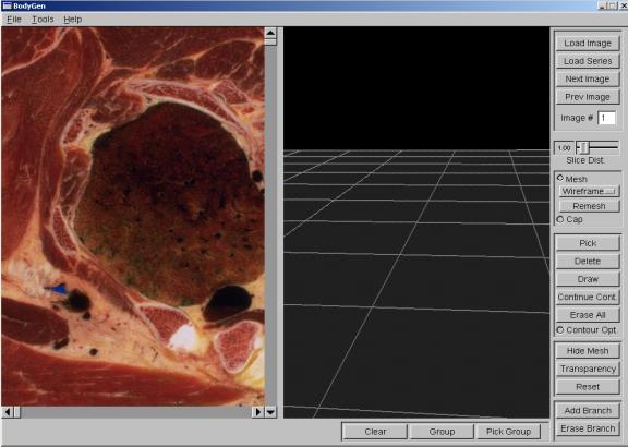
Figure A.1: BodyGen Screenshot

A.1 GUI Button Functionality

Load Image - This option allows the user to load in an image in bitmap format on which contours can be drawn. Assuming that n images are currently loaded, the next image will be loaded as image n+1 in the series.
Load Series - This allows the user to automatically load an entire series of images. Upon selecting this option a menu requesting, Base Filename, Start Number and End Number will be displayed. The base filename represents the starting string common to all files in the series, e.g. in the case of lung1.bmp, lung2.bmp, lung3.bmp, the starting string would be lung. Start and End Number represent the first and last image number in the series that the user wishes to load. Continuing the previous example, if lung1.bmp, lung2.bmp, ..., lung 45.bmp exist, but the user only wishes to load images 2-10, 2 and 10 would be entered here respectively. If the entire set is desired, these entries may be left blank.
Next/Prev Image - These buttons allows the user to cycle through the image planes currently loaded. As the names implies, Next and Prev Image cycle the current image up and down, respectively.
Image # - This text entry field allows the user to directly set the current image number.
Slice Dist - This slider allows the user to manually determine the distance between image planes. For a more accurate method of setting the slice separation, please see the Tools->Calibration entry.
Mesh - This checkbutton toggles the mesh display in the 3D view. When disabled, only contours and links will be shown, when enabled, the wireframe mesh for each ribbon will be displayed. When this button is activated, the user may choose between Wireframe and Smooth-Shaded using the drop down box below.
Cap - This checkbutton toggles the display of a cap covering the top and bottom of each object as a lid.
Remesh - During the course of modifying contour placement, contour vertex position, etc. ribbons may need to be remeshed. After contour modification, if the user feels that a mesh need to be modified to better represent the current contours, pressing this button will re-optimize the modified meshes.
Pick - This button enables picking in the 2D display. When an object is selected, mouse clicks in the 2D display will no longer draw contours, but instead select individual contour vertices. After selecting a contour vertex with the L mouse button, moving the mouse with the L button depressed will modify the vertex position. If multiple vertex selection is required, the user may click with the L button, and with the L button depressed draw a box around the desired vertices. Clicking on the red marker representing the center of a contour will automatically select all vertices of that contour.
Delete - This button (tied to the delete key as a shortcut) will automatically delete all selected vertices. If all vertices of a contour are selected, it will also delete the contour itself.
Draw - This button allows the user to exit Pick mode, and return to Draw mode where contours may be drawn.
Continue Cont - This button allows the user to continue adding vertices to previously completed contours. First, an entire contour should be selected in Pick Mode, next Continue Cont should be clicked. This will return the program to Draw Mode; however the next set of vertices that the user specifies will be added to the end of the currently selected contour.
Erase All - This button allows the user to erase all contours in the current image plane.
Contour Opt - This check button allows the user to minimize the number of vertices that are drawn, when a contour is specified. By examining the linearity of the curve drawn by the user, the program places only the minimum number of vertices needed to represent that curve. When not checked the program will place vertices at locations sampled from the curve drawn by the user at constant intervals.
Hide Mesh - This button operates on contours selected by the user in the 3D view. When pressed, the meshes associated with selected contours will not be displayed, even if the program is in Mesh Display Mode.
Transparency - Similar to the Hide Mesh feature, this button operates on contours selected by the user in the 3D view and when pressed, makes the meshes associated with selected contours appear as transparent in Smooth Shaded Display Mode.
Reset - This option returns the meshes associated with the selected contours to normal display, nullifying the effects of the Transparency and Hide Mesh buttons.
Add Branch - This button allows the user to manually add a link between contours on adjacent levels. After pressing this button, the user should select (with L mouse button and Alt key depressed) two contours on adjacent levels by selecting the center point of each contour in the 3D view. This will automatically add a link between the contours and generate the appropriate mesh.
Delete Branch - This button allows the user to manually delete a link between contours on adjacent levels. After pressing this button, the user should select (with L mouse button and Alt key depressed) two linked contours on adjacent levels by selecting the center point of each contour in the 3D view. This will automatically remove the link between the contours, and delete the corresponding mesh.
Group - This button allows the user to group together multiple mesh ribbons together into a single group. To group together a set of meshes, select the contours corresponding to the meshes in the 3D window, next click on Group with the left mouse button. A window will appear asking for the Group name. Upon pressing OK, the set of contours selected will become associated with that name.
Select Group - This button allows the user to quickly select groups of contours created with the 'Group' button above. Upon pressing this button a box will appear prompting the user to enter the group name. Pressing OK will automatically select the group of contours associated with that name.
Clear - This button clears the current selection in the 3D window and also cancels any pending Add/Erase branch commands.

A.2 Menu Item Functionality

File->Save Model - This option allows the user to save selected meshes in a .obj formatted file.
File->Save Contours - This option allows the user to save the current set of contours and branches to a file. All information pertaining to contour level, position, and links to contours in adjoining levels will be saved.
File->Load Contours - This option allows the user to load in work saved using the previous command. Note: Image data must be loaded before performing this operation.

Tools->Calibration - This option allows the user to set a correspondence between the scale of the image and the distance between image slices. The user is asked to draw a line on the image of a pre-specified length. This is used to determine the correspondence between pixels and mm. in the image. Upon selecting this option, the user will be presented with a menu requesting Draw Length and Slice Separation distance. Draw length is the distance represented by a line drawn by the user. Slice Separation Distance represents the distance between each pair of adjacent image slices.

A.3 Mouse Functionality

The mouse in the BodyGen application performs a number of different tasks depending on the current mode and window selection.

2D Contour Window (Draw Mode)
L Mouse Button – When depressed, BodyGen will begin to draw a contour. To outline a contour, move the mouse around the body of the desired contour with the left mouse button depressed. When contour is completed, releasing the L button will end the drawing of the current contour.

M, R Mouse Buttons – Not Used

2D Contour Window (Pick Mode)
L Mouse Button – If a contour centroid point (red circle in center of contour) is not selected, one vertex of a selection rectangle will be specified by clicking and holding the L mouse button. Dragging the mouse with the L button depressed will outline this selection rectangle. When the L button is released, all vertices within this selection rectangle will be selected, and can be deleted using the Delete GUI button. If clicking and holding w/ the L mouse button selects a contour centroid, all vertices of the chosen contour will be selected. Motion with the L button depressed will now move the entire contour.

M,R Mouse Buttons – Not Used

3D Contour Window (All Modes)
L Mouse Button – Motion of the mouse with the L button depressed will rotate the camera.

M Mouse Button – Motion of the mouse with the M button depressed will translate the camera.

R Mouse Button – Motion of the mouse with the M button depressed will scale the camera.

L Mouse Button + Alt – Left clicking on a contour centroid with the Alt key depressed will select all contours connected to the contour associated with the centroid.

L Mouse Button + Alt + Shift – Left clicking on a contour centriod with the Alt and Shift keys depressed will select the single contour associated with the centroid.

Appendix B

BodyView User’s Manual

This User’s Manual will introduce the novice user to the large number of user-interface features and commands in BodyView. We will detail each of these features and conclude with a brief tutorial on creating a scene from start to finish using the BodyView software. We will use the following screenshot from the BodyView application as a point of reference when discussing the available features.

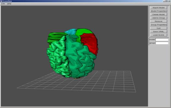
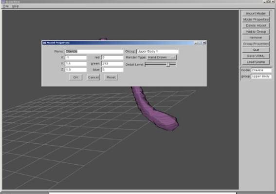
Figure B.1: BodyView Screenshot

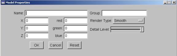
Figure B.2: Model Properties Dialog Box

B.1 GUI Button Functionality

Import Model - This button allows the user to load in a model in .obj format. Upon loading a model, the Model Properties dialog box (see Figure B.2) will appear, allowing the user to set model specific properties.
Model Properties – This button will display the Properties Box for the selected model. The Model Properties contain the following fields:

Name – Records the name of an object.
Group – Records the group in which the object will be placed.
X,Y,Z – Records the X,Y, and Z translation which will be applied to the object.
Red,Green,Blue – Records the R, G, and B color components for the model within the range 0-255. The model will be displayed in this color.

Render Type – Selects the Render Style for the current object.
Wireframe displays only the edges of the triangles composing the model. Smooth displays the object in the standard Phong shading style. Hand-Drawn1 will display the object using the multi-texture hatching NPR rendering method. This rendering scheme resembles a watercolor or oil painting. Hand-Drawn 2 will display only the silhouette lines of the object. This rendering scheme resembles a hand-drawn sketch of the object.
Detail Level – This slider selects the detail level for the current object. The far left position represent the coarsest detail level while the far right position represents the full detail original model. Selecting positions between these two extremes allows the user to fine tune the detail level of the object.
Reset – This button will return the X,Y, and Z translation parameters to 0.

Delete Model – This button deletes the currently selected model from the scene.
Group Properties – This button brings up the Group properties dialog box identical to the Model Properties dialog box described above except in one important respect; these properties act on all members of the specified group. For example, if Brain1 is entered in the Group field, and Hand-Draw 1 is selected, all rendering properties of the members of the Brain1 group will be changed to Hand-Drawn 1.
Quit – This button exits the BodyView program.
Save VRML – This button saves the current scene, as well as rendering and detail properties for each object, in VRML format.
Load Scene – This button allows the user to load a previously saved VRML file.

B.2 Mouse Functionality

The mouse serves both to manipulate the camera and reposition objects in the BodyView application.

L Mouse Button – Motion of the mouse with the L button depressed will rotate the camera.

M Mouse Button – Motion of the mouse with the M button depressed will translate the camera.

R Mouse Button – Motion of the mouse with the M button depressed will scale the camera.

L Mouse Button + Shift (no object selected) – Clicking on an object with the L mouse button with the Shift key depressed will select that object. A selected object will turn transparent purple, with a large white sphere present inside. (Note: the object’s rending property must be either Wireframe or Smooth for the object to become transparent.)

L Mouse Button + Shift (object selected) – Once an object is selected, clicking on the white manipulation sphere visible at the object’s center then moving the mouse will translate the object in the X, Z plane.

M Mouse Button + Shift (object selected) – Once an object is selected, clicking on the white manipulation sphere visible at the object’s center then moving the mouse will translate the object in the Y, Z plane. An object may be deselected by clicking away from the object with the L or M mouse button while the Shift key is depressed.